Algorithms Review
Spring 2017
Introduce the student to the concept of data structures through abstract data structures including lists, sorted lists, stacks, queues, deques, sets/maps, directed acyclic graphs, and graphs; and implementations including the use of linked lists, arrays, binary search trees, M-way search trees, hash tables, complete trees, and adjacency matrices and lists.
Introduce the student to algorithms design including greedy, divide-and-conquer, random and backtracking algorithms and dynamic programming; and specific algorithms including, for example, resizing arrays, balancing search trees, shortest path, and spanning trees.
Background
Data structures & algorithms govern the way we interact with digital information. At the highest level, they are used to organize and access abstract data types like containers (which store collections of objects).
Relationships & Orderings
The relationship between objects is often just as important as the information stored in the object. Most data structures can be described using the following six relationships:
| Relationship | Description | Examples |
|---|---|---|
| Linear order | Every object is strictly less than, equal to, or greater than another | Integers, hexadecimal memory addresses, alphabet |
| Hierarchical order | Each object has a parent object with the exception of the root object | *nix directories, single class inheritance (C#, Java) |
| Partial order | A hierarchical ordering with one or more root and no loops | Multiple class inheritance (C++), dependencies |
| Equivalence relation | Relationships where objects can be partitioned into subsets (equivalence relations) with other ‘weakly’ related (x~y) objects | 2n ~ 5n ∈ Ө(n) |
| Weak order | A linear ordering of equivalence classes |
O(1)< O(ln(n)) < O(n·ln(n))
|
| Adjacency relation | Relationships described by an object being connected to another (x ↔ y) | Graphs, social networks |
Asymptotic Analysis & Big-O Notation
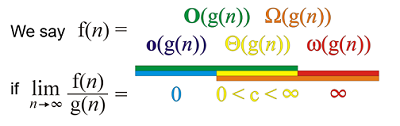
It’s often useful to analyze and compare algorithms with respect to one or more variables (i.e. run-time, memory). Using the same ‘Big O’ mathematical notation and Landau symbols used to describe the limiting behaviour of a function, the efficiency of different algorithms can be compared. For two algorithms described by the functions f(n) and g(n), the best- and worst-case behaviour of the algorithms can be described as such (n can be a measure of run-time or memory):
-
f(n) = o(g(n))whenf(n)approaches ∞ at a slower rate thang(n)(f outperforms g) -
f(n) = O(g(n))whenf(n)approaches ∞ at a rate equal to or slower thang(n)(f, at worst, performs the same g) -
f(n) = Ω(g(n))whenf(n)approaches ∞ at a rate equal to or faster thang(n)(f, at best, performs the same g) -
f(n) = ω(g(n))whenf(n)approaches ∞ at a much slower rate thang(n)(g outperforms f) -
f(n) = Ө(g(n))whenf(n)andg(n)approach ∞ at comparable rates (f and g perform roughly the same)
Note that since this notation describes limiting behaviour, one should be wary of making objective statements about the relative performance of two different algorithms without context. For example, even though f may run faster than g for n = 1000000, the opposite could be true when the same algorithms are run on only 1000 objects. Similarly, since Big-O notation gives information about the relative scaling and complexity of different algorithms rather than their absolute performance, for an algorithm f that scales faster than another, g, by a constant factor, f(n) = Ө(g(n)) is still true.
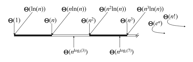
After taking these caveats into consideration, Landau symbols prove very useful for describing the complexity of an algorithm. An algorithm is considered to run in polynomial time if its run time can be described by O(n^d) for d greater than or equal to zero. Algorithms with polynomial time complexity are considered efficient in the current non-quantum state of computing, whereas problems that can not be solved in polynomial time are considered intractable or infeasible (e.g. the traveling salesman problem). Although these problems could still theoretically be solved, the scaling is computationally inefficient enough that it is typically not worth the effort except for special cases of the problem.
Linked Lists
Linked lists are the simplest type of data structure, consisting of a set of linearly ordered nodes that, in addition to storing data, also contain an address pointing to the location next node in memory.

- Pros: Simple,
O(1)insertions w/out reallocation - Cons: Inefficient indexing, poor cache locality
Project 1: Doubly Linked Sentinel List
Complete? Description Grade <Type> templated linked list w/a second sentinel at the end (for improved indexing/insertion at the back of the list) and O(1) copy & move constructors 24/24 (100%)
Stacks , Queues, & Deques
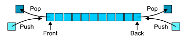
The stack data structure are most commonly used as data buffers. Being linearly ordered, stacks are often implemented using a wrapper class around a linked list, and as such retain much of the functionality of a list structure. However, rather than manually traversing the list, member functions for stack/buffer data structures are typically limited to two principal operations that insert (push) and remove (pop) an object onto/from the stack.
Traditional stacks display last-in-first-out (LIFO) behaviour meaning the first object pushed onto the stack cannot be popped until all of the objects pushed after it have been popped - like a stack of books. Stacks with a first-in-first-out (FIFO) behaviour are called queues (for reasons that should be self-evident). Apart from the obvious applications (waiting in line at the bank), queues more generally used in client-server models where the server must handle a large number of service requests from clients. Finally, the deque abstract data structure allows an objects to be pushed to the front or the back of the list meaning it can be used as either a queue or a stack.
Other Considerations
Despite being a relatively simple data structure, efforts to optimize the efficiency of real-life implementations can be very complicated. For example, stacks and queues can also be implemented efficiently using dynamic arrays. Whereas prepending to a linked list is always O(1), appending elements to an array list is amortized O(1) meaning although the total time for n insertions is O(n), the time bound of any individual insertions can be much worse. This is a result of the cost of resizing a full array and reallocating contiguous blocks of memory. Conversely, unlike linked lists which usually require O(n) memory to store pointers in each node, the memory overhead for a dynamic array is typically O(1) (only approaching O(n) after the array capacity is doubled). Other examples of stack-based structure implementations include queues with dynamic array used as a circular buffer, priority queues, and other more esoteric structures like hybrid VLists.
Project 2: Resizable Deque
Complete? Description Grade <Type> templated resizable deque structure. Capacity of circular array is doubled when push is called in a deque overflow state resulting in amortized. O(1) push operations 28/28 (100%)
Trees
Perhaps one of the most widely used and versatile data structures is the hierarchically-ordered tree structure consisting of a root node (with no superior) and subtrees of children that succeed it (each with a superior parent node). The degree of an individual node refers to the number of children succeeding that node, with a node with degree zero referred to as a leaf node. There exists a unique path from each node in a tree from the root node to that node, the length of which is referred to as the depth of the node. The height of a tree is defined as the maximum depth of any node in the tree. Like stacks, tree data structures can be implemented using a collection of linked lists (with nodes containing addresses of the parent node and its children), or by cleverly taking advantage of the contiguous memory allocation of arrays. Traversing these trees in order is typically accomplished using a stack (breadth-first) or using recursion (depth-first).
N-ary trees
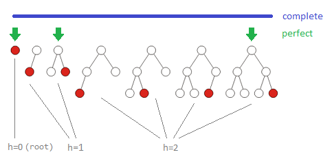
An N-ary tree is a tree with each node containing at most N sub-trees. Each node of a binary search tree, for example, contains at most two children normally referred to as the ‘left’ and ‘right’ child. In a ‘perfect’ N-ary tree, every node has exactly two children except for the nodes at the maximum depth (bottom layer) of the tree which are leaf nodes (with no children). A ‘complete’ N-ary on the other hand, must be filled from left to right meaning the tree is perfect except for the leaf nodes a the deepest level (which may or may not be filled).
A perfect N-ary tree with height h will by definition always contain n=(Nh+1-1) / (N-1) nodes, which for a binary tree simplifies to 2h+1-1 nodes. Rearranging for the height, h we find h= logN(n(N-1)+1)-1 which is typically approximated as h =~ logN(n). This proves important for run-time analyses of operations on trees, which are usually O(h). For example, because order is preserved in complete binary trees, they can be used to store sorted lists where every node of a left sub-tree contains elements strictly smaller than the root element, and every node of a right sub-tree contains elements strictly greater than the root element (known as a binary search tree). Unlike arrays and other sorted list structures with O(n) operations, finding and inserting elements in a binary search trees only requires an O(h) depth-first (recursive) traversal of the tree. Note that operations on a worst-case unbalanced tree with h=n (essentially a linked list) will still be O(n).
Balanced Trees & Other Tree Data Structures
Given the importance of tree height on their performance, it’s no surprise extensive efforts are typically made to optimize the height of tree structures. Although the best-case scenario of a perfect tree (in which the descendants of each nodes are perfectly balanced) is not always achievable their are a variety of algorithms available that aim to balance trees using different criteria. AVL trees use a height balancing algorithm that compares the height of child sub-trees to determine whether the tree is in a state of in balance before performing a series of rotations to restore balance.
A binary heap also uses the binary tree structure, and are frequently used to implement priority queues. The distinguishing feature of a min-heap is that every child contains a key less than or equal to its parent (and vice versa for max-heaps). A B+-tree is another example of a balanced N-ary tree with a variable (and typically large) number of children for each node that is particularly useful in retrieval of block-oriented storage contexts (i.e file systems). Finally, unlike an N-ary tree, a multi-way (M-way) search tree can store M-1 elements and can have up to M sub-trees.
Project 3: AVL Search Tree
Complete? Description Grade <Type> templated, self-balancing binary search tree w/iterator protected nodes 16/16 (100%)
Sorting
At a fundamental level sorting involves taking an abstract list containing unsorted objects and converting it into a list of linearly ordered objects (an Abstract Sorted Lists). These operations are typically performed on arrays since they are the data type most commonly used for storing. Every sorting algorithms rely on the the following five techniques: insertion, exchange, selection, merging, or distribution. In-place sorting algorithms can perform this conversion without making a second copy of the list in memory meaning memory allocation is Ө(1) at most. In terms of run-time efficiency, sorting algorithms fall into three different categories: Ө(n), Ө(n·ln(n)), and O(n^2), depending on the degree of unsortedness in the list an other factors. Of course, since every sorting algorithm must inspect every one of the n elements being sorted at least once, there is a Ω(n) lower bound on the run-time of sorting algorithms (Ω(n·ln(n) being more realistic in most scenarios). The following descriptions assume elements are being sorted in ascending order from left to right.
O(n2) sorts
-
Insertion sort starts from the second element in an array and compares it to the element to its left (using nested
forloops). Under the condition that the element to its left is smaller, the current element is swapped with the lesser element until this condition is no longer true, at which point the current element is updated to the next unsorted object. As a result, after k iterations, the first k elements will be sorted. Subsequent iterations will insert an element from the unsorted section (right side) of the list into the sorted section (left side) of the list. Insertion sort is an online algorithm meaning it can sort a stream of inputs without knowing the final size of the list.
Animated illustration of an insertion sort
-
Bubble sort uses the opposite strategy; the first element is swapped with the element to its right until the element to its right is greater than the current element. After k iterations we are only guaranteed the right-most (largest) k items will be ordered. Unlike iterations of insertion sort (which terminate early when the current element finds its sorted position), every iteration of bubble sort requires every element in the unsorted section of the list be compared with its neighbor with no opportunity for early termination. This gives insertion sort an advantage when it comes to partially-sorted lists. Moreover, because bubble sort relies on assuming the right-most element is always the global maximum, it is not an online algorithm meaning the algorithm, requiring bubble sort to restart every time an item is added to the list.
-
Selection sort, closely resembles insertion sort, but searches for the smallest unsorted element at every iteration before moving it to the (sorted) front of the array (rather than sorting the left-most unsorted element in each iteration) making it slightly less efficient than insertion sort.
Ө(n·ln(n)) sorts
-
Heapsort is the simplest of the
Ө(n·ln(n))sorting algorithms and the only one that can be performed in-place (O(1)overhead). As the name implies, a heapsort transforms an unsorted list into a heap. This heap is converted to a max-heap meaning the largest (right-most) element in the sorted array will always be at the root of the heap. The element at the root node is then swapped with the element at the end of the heap before being removed from the heap entirely. At this point the heap is converted to a max-heap again, and the process repeats until the heap is empty. Because heapsort relies on a tree data structure, it is guaranteed to beӨ(n·ln(n))even for very large inputs while also maintaining a constant upper bound on memory overhead. -
Quicksort is a recursive nearly-in-place sorting algorithm which is in most cases faster than heapsort. Quicksort chooses an element in the unsorted array as a pivot and splits the remaining elements into to two groups - one with elements less than the pivot, and the other with elements greater than the pivot. The pivot is moved to the middle of the array, and quicksort is called recursively on the sublists on either side of the pivot. A simple insertion sort is often used as the ‘base case’ for the recursion once the sublists being sorted are small enough. Although efficient implementations of quicksort have low memory overhead and are faster than heapsort on average, the worst-case scenario where the chosen pivot does not evenly divide the unsorted list can result in
O(n^2)run-times which can be particularly problematic for very large inputs and leaves critical/secure applications relying on quicksort vulnerable to attack from a malicious party with a detailed understanding of the algorithm . The median-of-three strategy attempts to minimize the risk of running into the worst-case scenario by using the median of three (sometimes more) numbers from the beginning, end, and middle of the unsorted list as the pivot (with no significant effect on runtime). -
Merge sort is an example of a stable divide-and-conquer sorting algorithm, meaning identical inputs are sorted in th same order than they appear in. Instead of using the value of an element to divide an unsorted list like quicksort, merge sort splits the larger problem into two sub-problems based on location in the array (typically the midpoint). Merge sort is called recursively on each sublist either until the sublist contains a single element or until it is small enough to be sorted using insertion sort efficiently, depending on the implementation. Elements of sorted sub-lists are then compared and merged together to form larger sorted lists until every element has been sorted. Because it is impossible to merge two arrays in-place, merge sort has an Ө(n) memory requirement that sets it apart from quicksort and heapsort.
Ө(n) sorts
- Bucket sort and radix sort need to make assumptions about the data being stored in order to achieve run-times better than Ө(n·ln(n)). Both algorithms work best for inputs that are uniformly distributed over a known range, such as floating point numbers. Both algorithms create buckets (or bins) spanning the range of expected inputs before stepping through the unsorted list and placing each element in the unsorted array into their appropriate bucket. Bucket sort completes the sort by stepping through buckets (which span the entire range of possible values) in order and rebuilding the list in order using only filled buckets, whereas radix sort uses the results from the first iteration of bucketing by least-significant digit to ‘re-bucket’ the elements by the next-most-significant digit. These distribution-based sorting algorithms have low memory requirements (depending on the range of the data) and fast run-times, although it ultimately depends on both the number of objects, n, and the range of the data stored in the objects, m.
Summary: Sorting Algorithms
The following table compares the algorithms discussed in the previous sections and details their individual run-time complexities. More sophisticated variations of these algorithms like Timsort, introsort, and shell sort are built using the core principles of these sorting algorithms.
| Algorithm | Best | Average | Worst | In-place? | Usage/Distinguishing Features |
|---|---|---|---|---|---|
| Selection sort | Ω(n^2) |
Ө(n^2) |
O(n^2) |
Easy to implement | |
| Bubble sort | Ω(n) |
Ө(n^2) |
O(n^2) |
Easy to implement | |
| Insertion sort | Ω(n) |
Ө(n^2) |
O(n^2) |
Ideal for small n, online (streamed) lists | |
| Heapsort | Ω(n·ln(n)) |
Ө(n·ln(n)) |
O(n·ln(n)) |
Main concern is worst-case performance/memory | |
| Quicksort | Ω(n·ln(n)) |
Ө(n·ln(n)) |
O(n^2) |
Fastest but sometimes slowest, nearly in-place | |
| Merge sort | Ω(n·ln(n)) |
Ө(n·ln(n)) |
O(n·ln(n)) |
Fast + stable, but O(n) overhead | |
| Bucket sort | Ω(n+m) |
Ө(n+m) |
O(n^2) |
Ideal for evenly distributed data | |
| Radix sort | Ω(n·m) |
Ө(n·m) |
O(n·m) |
Ideal for n>>m (m = range/# of radix digits) |
Hash Tables
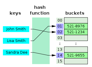
Hash tables (sometimes called hash maps) are a data structure designed to store key/value pairs, the classic example being a name (key) and phone number (value). They are, by design, particularly efficient for ‘lookup’ operations - even more efficient than search trees - and consequently are widely used in caching and indexing related applications. A perfect hash table uses a hash function to generate a unique hash for every key, which is then mapped to a specific index of an array of buckets. This ideal table stores data so that all operations have Ө(1) time complexity and require at most Ө(n) memory overhead. In reality, most hash functions have a non-zero chance of generating the same index for two distinct keys (a hash collision) and allow insertions and deletions at amortized constant average cost per operation.
Hash functions
An efficient hash table requires a hash function that is fast and deterministic (meaning it always returns the same hash for any given key). For a 32-bit integer hash, two random objects should have a 1/232 chance of having the same hash value. Finally, for objects that are conceptually equivalent (e.g. 1/2 and -1/-2) will ideally have the same has value. Predetermined hash functions use a value that is explicitly assigned to an object. Examples are the address of an object in memory, or an unique assigned ID like a social insurance number. Although convenient, explicit hash values often run into problems - for example, identical strings stored in two different variables would have different addresses in memory despite being conceptually the same.
The obvious solution is to derive a hash function that depends on the input and its member variables. Arithmetic functions are the most common implementation of these ‘implicit’ has functions. Depending on the application, simple manipulations of the integer returned by casting an object as an integer (e.g. static_cast<unsigned int> in C++) are usually enough to generate a fast Ө(1) hash function with an even distribution and minimal chance of collision. Mapping this integer into an integer within the allowed indexing range for the array is easily accomplished using the modulo operator (%) and, in the case where the array size is a power of two, the remainder operation is reduced to masking (resulting in improved speed).
Collision Resolution
Hash collisions are considered in most implementations of the hash table data structure are considered an inevitability for the same statistical reason that the birthday paradox arises. As Wikipedia states:
if 2,450 keys are hashed into a million buckets, even with a perfectly uniform random distribution, according to the birthday problem there is approximately a 95% chance of at least two of the keys being hashed to the same slot
Consequently, the way a hash table data structure handles collisions is typically where implementations differ the most. Collision resolution strategies usually fall into two categories: tables with separate chaining, and those with open addressing. Separate chaining is the simplest approach, with each bucket in the array corresponding with a liked list. When an objects is assigned to a bucket already containing an object the push operation is called on the linked list in that bucket to extend the list. As the length of these linked lists grows, eventually the access times will start to increase - one of the reasons that a good has function with a uniform distribution is important. The load factor λ = n/M is used to describe the average number of objects per bucket and is directly related to the access time. An obvious disadvantage of using a linked list (and even implementations that use tree structures instead) with chained hash tables is that it requires a significant amount of dynamic memory allocation as the table grows.
Open addressing circumvents this by following a predefined sequence of bins to search after a hash collision so that instead of using dynamic memory to store objects with matching has values, unused space in the contiguous block of memory reserved for the array is used. As a result, has tables with open addressing will never have a load factor greater than unity and are typically more efficient. Open addressing using linear probing is the most straightforward strategy; assuming an object is being inserted into bin k, linear probing dictates that the algorithm attempt to insert the object in bin k+1 if bin k is full. If bin k+1 is full, bin k+2 is the next bin searched, and so on. Unfortunately, primary clustering as a result of this probing process can result in quickly increasing access timesNote that a hash table with open addressing requires each object be re-hashed each time the array is resized. This can be mitigated using quadratic probing, which uses the same strategy but uses a searching sequence that progresses quadratically instead of linearly. For an array with M = 2m bins using the rule bin = init_index + (k + k*k)/2 (where k is the loop iteration counter) is guaranteed to visit every bin once before repeating and results less problematic in secondary clustering instead of primary clustering.
Project 4: Quadratic Hash Table
Complete? Description Grade <Type> templated hash table with open addressing (quadratic probing) and Ө(1) operations for load factors < ~0.666 8/8 (100%)
Graphs
The graph data type and the undirected and directed graph data structures that use it borrow from the field of graph theory in mathematics. Graphs consist of a finite number of nodes (also called vertices) connected by edges that are used to associate nodes with each one another. Graphs are represented formally using a pair of sets (V,E) where V is the set of vertices and E is the set of edges that link the vertices together. In an undirected graph, edges are always symmetric meaning x → y AND y → x whereas in a directed graph the direction must be specified. Some graphs also assign an edge value or weight to each edge representing, for example, the cost a of transition from x → y.
A graph is considered a tree if it is connected and there is a unique path between any two vertices. A tree will, by definition, have one less edge than it does vertices and not contain any cycles - adding just one more edge breaks this property. The degree of a vertex refers to the number of adjacent nodes to which it is connected. In the case of a directed graph, the in-degree and out-degree is used to specify the the number of edges ‘entering’ the node and the number of edges ‘leaving’ it, respectively. Vertices with an in-degree of zero are described as sources, whereas vertices with an out-degree of zero are described as sinks.
A directed acyclic graph (DAG) refers to a graph that is both directed and also does not contain any cycles. Besides being well-defined, DAGs have a number of useful properties that make them useful in a variety of applications. Among these applications are dependency graphs formed by inheritance relationships in object-oriented programming languages, and file systems. Implementations of any type of graph data structure must decide on how the adjacency relationships that comprise the graph are stored. The simplest solution, the binary-relation , which uses a container with a list of pairs representing each individual connection is the least efficient solution. An adjacency matrix uses each entry of a V x V matrix to store connections, with each cell (i,j) containing information about the edge from node i to node j . Although adjacency matrices are more efficient than binary-relations, graphs are most efficiently implemented using an adjacency list where every vertex is associated with a list of its neighbors. Adjacency matrices are still preferred, however, if the graph is dense ( E ~ V^2).
Topological Sorts
The partial ordering that represents a dependency graph (or any other DAG) can be sorted topologically in linear order such that Va appears before Vb only when there is a path from Va to Vb. In the case of a dependency graph, a topological sort provides a feasible schedule or order in which every node can be visited without breaking any dependencies. Since every DAG has at least one source (a node with an in-degree of zero) and no cycles, every DAG and its sub-graphs must also have a topological sort. Topological sorts are usually implemented using a queue initialized with all source vertices and an array containing the in-degree of each vertex in the graph. Starting with the first vertex in the queue, nodes are popped one-by-one until the queue is empty, with the in-degree of each one of the nodes adjacent to the node being popped being decremented each time. Once the in-degree of a neighbouring reaches zero, it is pushed onto the queue. The order of the nodes popped from the queue defines the topological sort.
In the case where there is a weight associated with each edge, it is also useful to find the critical path, that is the longest path from the first node (or, in project scheduling, milestone) to the last. For example, a dependency graph where each weight represents the time required to complete the task represented by each vertex, the critical time would represent the longest, rate-determining sequence of tasks that cannot be parallelized with respect to each other (any delay to tasks this sequence will delay the overall task).
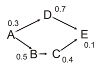
Path A → D → E with length 1.1 is shorter than path A → B → C → E with length 1.3, but since E requires C, the longest path is considered the critical (rate-determining) path
For our topological sort algorithm, if, in addition to the in-degree, we use arrays to keep track of the critical time and previous task for each node (initialized to zero/null) and, every time a vertex is popped:
- add the task time (edge weight) to the critical time for that vertex
- if the new critical time exceeds the critical time of any vertices adjacent to the popped (source) vertex, replace those neighbours’ critical time with the new critical time and point their previous task to the popped vertex the order of the topological sort will also be the shortest critical path of the DAG.